• Surge and storms in the south
• A jumpy IOD forecast – is this the predictability barrier at work?
• Strange buoy behaviour at 47 S

SST update

Warm anomalies have increased this week off NSW due to two warm core eddies: one very strong eddy east of Gabo Island, and another about 180 nm offshore of Sydney. This second eddy is drawing the main arm of the East Australian Current down to 36 S before it retroflects back to the north and the east.

IOD jumps up

The latest IOD outlook has jumped into a strong positive event. Climatologists are now more confident that these conditions will continue for the rest of the year.

As discussed last week, the ACCESS-S ensemble was showing a weakly positive pattern on average. But the latest outlook has firmly moved into the red.

The ACCESS-S model is the BOM’s new seasonal prediction suite and is known to do well in predicting the occurrence of IOD and ENSO events.

However, the skill in intensity is still being worked out.

So how predictable is the IOD?

Studies show there may be two predictability barriers for the IOD. One in summer and one in winter. The austral winter barrier is thought to be in May (Shi et al 2011).

The forecast skill of SST in Indian Ocean is known to be less than in the Pacific Ocean, with the eastern Indian Ocean being the hardest to predict. Shi et al (2011) studied several global models including BOM’s POAMA (the predecessor to ACCESS-S) and found there is good skill in predicting a September IOD event 3 months in advance with a 60-80% hit rate. Stronger events can be predicted up to 6 months in advance. But on the other hand, there is also a high false alarm rate of over 50 %.

These numbers are not great. Especially compared to ENSO forecasts.

The authors suggest that the IOD forecasts are too volatile because modelled thermocline depths in the equatorial eastern Indian Ocean are too shallow.

Another study found that this predictability barrier is caused due one of two types of errors in the initial conditions (Liu et al (2018) :

1. A large negative SST anomaly in the central eastern Pacific and an associated subsurface pattern.
2. The same but with the opposite sign.

These anomalies affect the wind in the eastern IOD box and thus the SST forecast. The authors found that whatever the start month, the forecast skill decreased rapidly over the austral winter.

A recent paper goes further and claims that there is a SST error dipole. Feng and Duan (2019) found that the initial errors in the Pacific Ocean are linked to the Indian Ocean by an atmospheric bridge. Thus initial errors on either side of the Maritime Continent can cause a predictability barrier.

So what?

Well, we need more in-situ observations in the tropical Indian Ocean to reduce SST bias in the models.

And for now we need to take any forecasts beyond 3 months with a grain of salt.

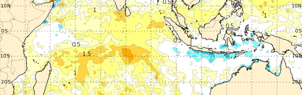
Here is the current state of the SST anomalies in the two IOD boxes.

Is looks weakly positive. And we have left behind the May predictability barrier by at least a month. But will the prediction of a strong positive event continuing beyond September turn out to be a false alarm? We will see.

Storms and surge in the south

Wild weather is battering the southeastern part of the country, with gale forces winds, heavy rain and elevated snowfalls across SA, VIC and TAS.

The first front crossed on Wednesday night, but a stronger front is due on Friday evening.

Media outlets are warning of cold ‘feels like’ temperatures, polar conditions, wild winds, and blizzards. 

BOM is also trying to reach out to the public via Twitter in the absence of official hazardous surf warnings for southern states. (A service only currently implemented in NSW and QLD).

There is an associated surge in sea level. OceanMAPS predicts the surge could reach 0.5 m along parts of southern Victoria, and even up to 0.7 m in the north end of the Spencer Gulf on Friday.

On Wednesday night a tidal residual of 1.0 m was measured at Cape Jervis.

The surge will peak on Friday and then move as a coastally-trapped wave anti-clockwise around the country. Sea levels greater than HAT are expected in NSW on Sunday and southern QLD on Monday.

As the CTW water surges around the corner, coastal currents will strengthen… and ready to meet the CTW on the eastern corner of VIC is a strong warm core eddy!

We could see 3 knot currents going in opposite directions only a few miles apart. The sea state off Gabo Island is likely to be very difficult for mariners over the weekend.

Thinking of the deeper ocean now … how are the strong winds and wave affecting the stratification of the ocean?

Along South Australia and into the Bass Strait the injection of very strong momentum flux is not forecast to change the mixed layer depth. The water is already well-mixed to the seabed and the MLD reflects the bathymetry. In contrast, on the southern NSW coast the MLD depth is reflective of the eddy pattern of the East Australian Current.

A mysterious drifter

A drifting buoy is behaving strangely in the southern Tasman Sea.

Why is it going around in 3 km wide circles? 

The mysterious buoy became the subject of interest when it was spotted on the iQuam website.

Can there really be a mooring out there? The bathymetry is 4700 m deep.

The buoy ID number corresponds with Canadian moored buoys. That doesn’t seem right. How do we tell what type of instrument it really is?

The GTS messages coming in from the buoy look like this:

For those that don’t know BUFR tables by heart the messages say the buoy has a 15 m drogue that is attached.

• Drogue Type 1 = Holey sock
• Drogue Depth = 15 m
• Lagrangian Drifter Drogue 1 = Attached.

A drifting buoy makes a lot more sense in this part of the world. But mystery continues – the circles are too large for a moored buoy, but too small for a drifting buoy, especially on the edge of the Southern Ocean where one would expect drifting buoys to head eastward.

Perhaps there is a strong eddy pulling the drogued buoy around in circles. Let’s look at OceanMAPS currents ensemble at 17.5 m depth.

There is nothing obvious in the velocity field, and the standard deviation is small.

So the strange circular behaviour is yet to be explained.

Do you know any more clues to this oceanic mystery? Please leave a comment.