
- North coast cools rapidly but NSW eddy pair continues hot
- East coast surge in sea level next week
- Observations of an eddy pair from the RV Investigator
SST update

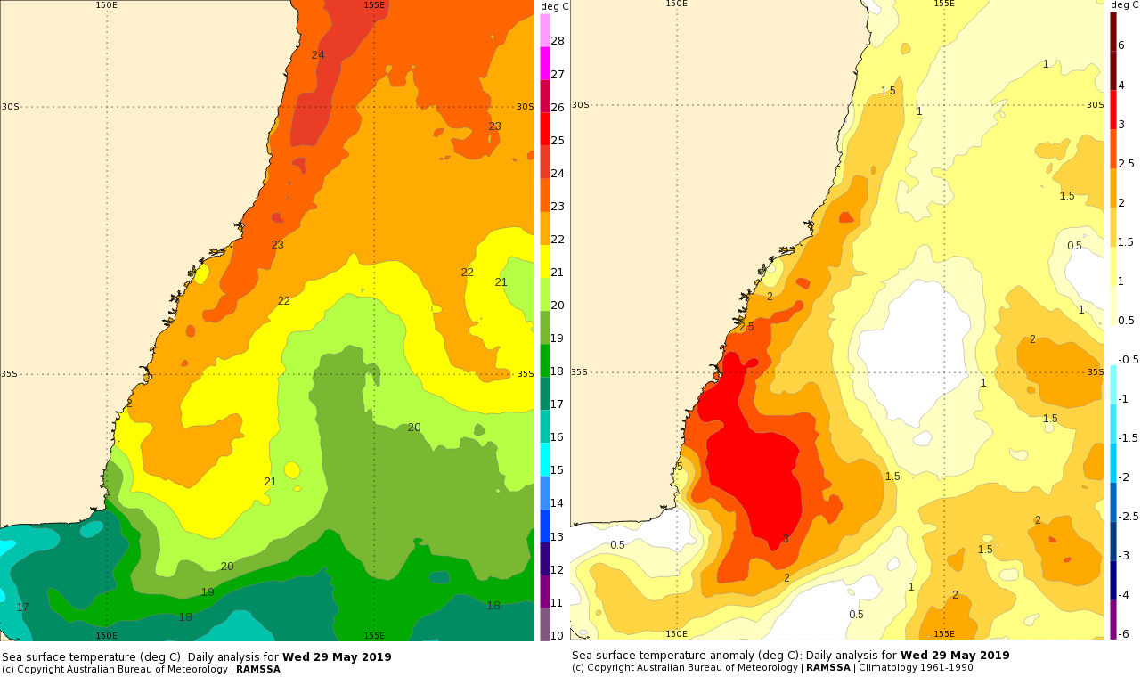
There have been incremental changes in the SST anomaly pattern this week. The main driver has been a series of cold fronts that crossed the south of the country, with high pressure establishing behind. This weather has fed cool air a long way north with many places experiencing air temperatures 4 to 8 deg C below normal.

The cool air will also affect sea surface temperatures, accelerating seasonal cooling. This is particularly noticeable in the north of the country. We have already seen the start of the winter production of cool inshore water but this week the effect will be amplified.
In the southern Gulf of Carpentaria OceanMAPS is predicting a drop in SSTs from 24 deg C down to 22 deg C within a few days.

Meanwhile, the warm anomalies over NSW have not eased at all despite forecasts last week.
Did the OceanMAPS forecast actually pan out?
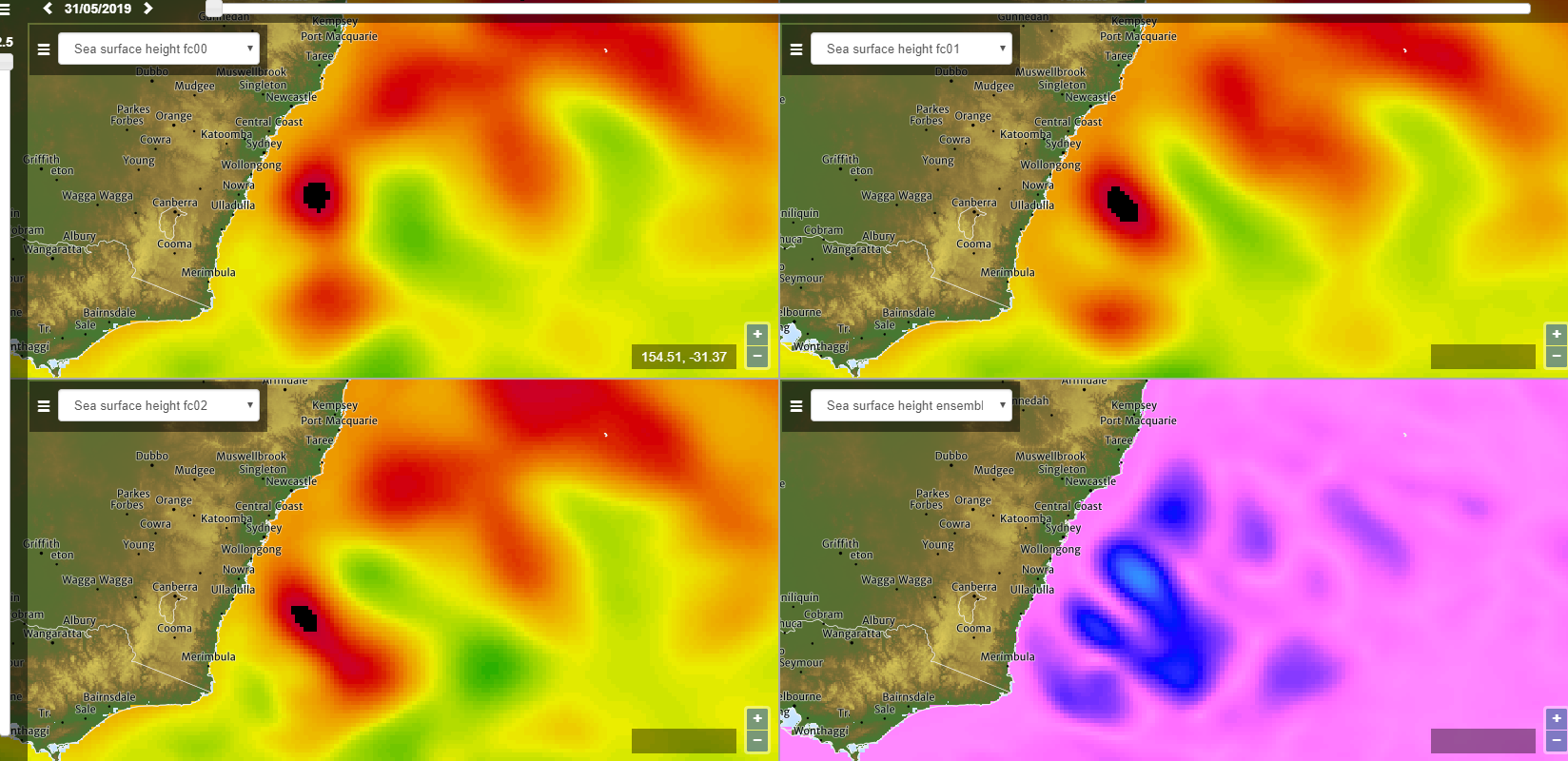
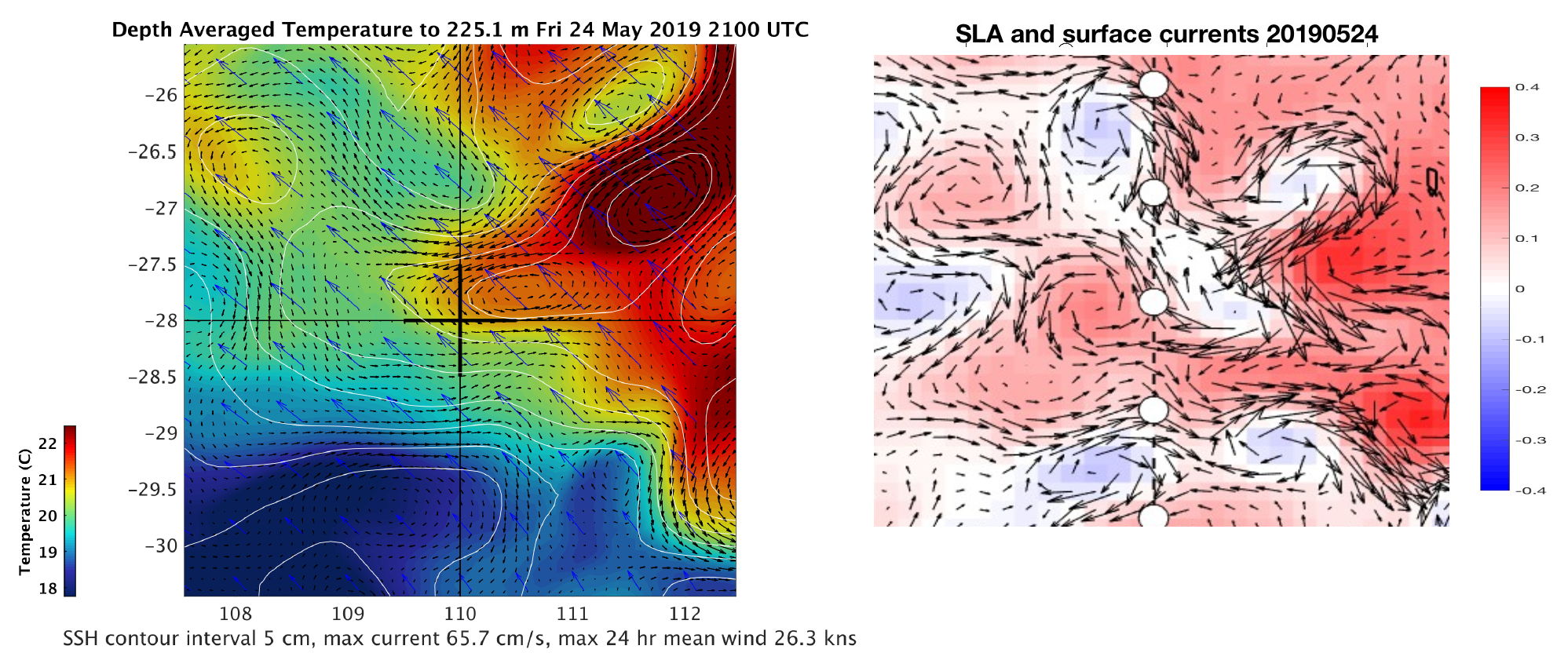
Let’s compare the 7-day forecast for NSW with the model result on the day. Eyeballing the left and right images below, we can see that there is broad agreement about the behaviour of the warm eddy off southern NSW. Some of the warm water of the main eddy has ‘leaked’ southward and joined a secondary eddy. The difference is that the long range forecast kept the southward eddy weak and the two features distinct, while the latest forecast has the eddies both quite strong and joined together with a larger area of 22 deg C water.

You can check out the eddy structures in the latest SLA images here.
In fact, model uncertainty continues. The images below show the three sea surface height (SSH) solutions in the OceanMAPS ensemble, with the bottom right image showing the ensemble standard deviation.
The dynamics of this eddy pair, separate or apart, will have direct influence on the longevity and location of the SST anomaly. We’ll have to wait and see how this plays out.
Surge up the east coast
A low pressure system is expected to form in the Tasman Sea by Monday. This will generate strong southerly wind and large waves up the eastern seaboard.

This situation has many forecasters reaching for the Aggregate Sea Level Viewer.
Many red alerts of sea level above HAT are showing along NSW and southern QLD. The combination of a southerly surge and spring tides is particularly worrisome.

Most exceedence levels are small at this stage. Many stations show sea levels only 5 cm above HAT on Tuesday and Wednesday next week. However, some stations are higher with the maximum ensemble member at Noosa QLD showing 20 cm and Forster NSW showing 30 cm exceedence.
Wave setup will be another important component. At the moment we are too far out for the National Storm Surge model that includes wave setup – this only goes out to three days. AUSWAVE-G suggests the significant wave heights could be as big as 6 to 7 m offshore, with a 12 second period. It is highly likely that Dangerous Surf warnings will need to be issued.
On the other side of the country, spare a thought for the Margaret River Pro surfing competition who had to postpone competition yesterday due to a lack of waves.

Luckily, a long period swell will arrive from the west tonight (Friday) and should lead to good contests over the weekend. Check out the swell forecast here.
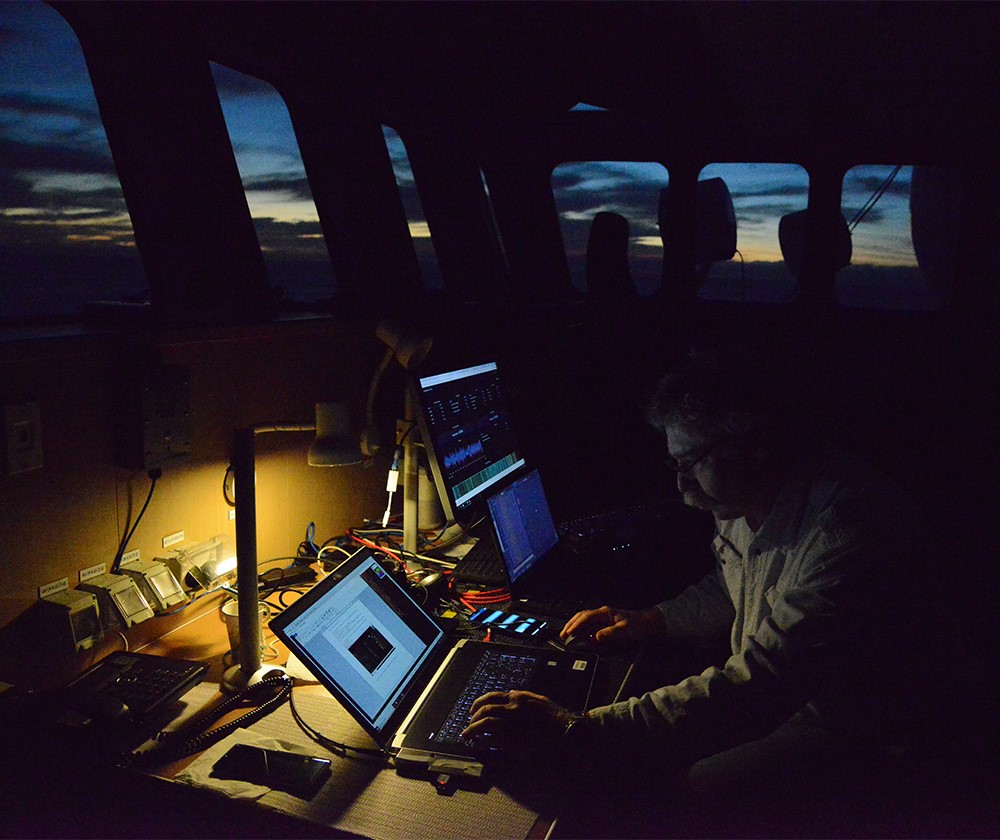
Observations from RV Investigator
We have received some feedback about OceanMAPS from the RV Investigator. As mentioned last week the research vessel is tracking along the 110 E line and conducting oceanographic measurements.

One of the daily logs reads: “The ship operates on a 24/7 basis and most of the scientists are on 12-hour shifts, which rotate at 2am and 2pm. The 2am shift has a few hours of steaming until the ship reaches the location of the next station and, as we are approaching it, a sonobuoy is deployed, the Continuous Plankton recorder is retrieved, and by 7am the CTD is descending to the inky depths of the Indian Ocean. This takes several hours as the seafloor is generally deeper than 5,000 m! As the CTD returns to the surface, the Niskin bottles are fired to collect water at the different depths as per the water budget. When the CTD is back on board there is an intense period of emptying of the Niskin bottles so that everyone can get the water they require for samples and experiments.” – Prof Lynnath Beckley.
After one of the routine CTDs on the 25th of May, Dr Helen Phillips from the University of Tasmania wrote to the BOM to note:
Usually the [OceanMAPS] current direction has been matching quite well with what we see on the shipboard ADCP.
Today was a bit unusual in that we were experiencing flow towards NNW during the 4 hour CTD while the nowcast was showing currents from the ENE.
The measured current direction matched up better with the Copernicus forecast that the ship was using as a comparison model.
What was going on?
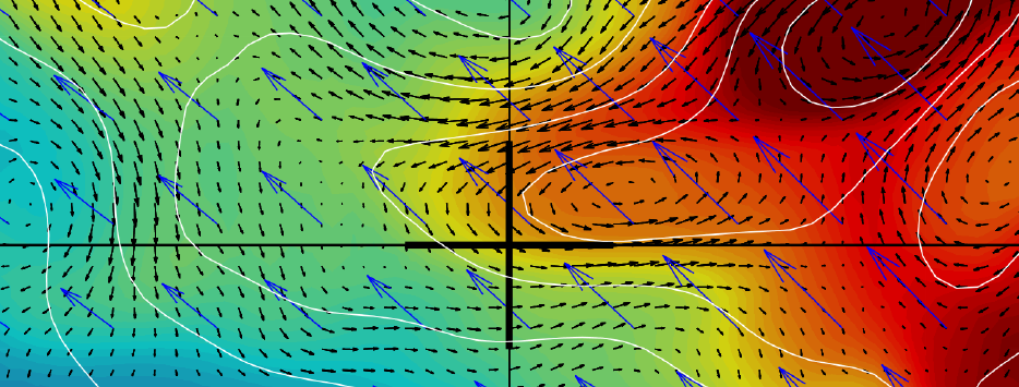
It seems that the two models disagreed about the position of a pair of warm eddies. OceanMAPS had the eddies joined, while Copernicus had them separated. See below.
From what we could see in the maps:
- The strong warm eddy at 27 S and 112 E matched up in both models.
- The secondary warm eddy to the southwest was at 27.7 S 110.7 E in OceanMAPS but at 27.7 S 109.5 E in Copernicus.
- If the two eddies were separate there would be a flow towards the north-northwest on the 110 E line (as was observed).
In fact, OceanMAPS corrected itself on the very next run.
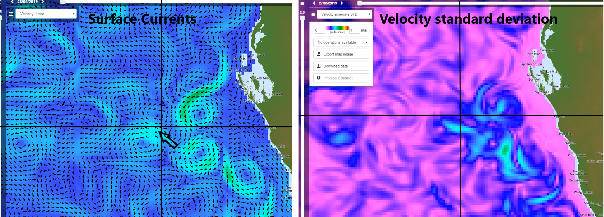
The two eddies were indeed separate. The ensemble standard deviation plot shows the large uncertainty in that region. The Leeuwin Current is at full strength and spawning eddies at this time of year. It is a dynamic time.
Observations from the field help pinpoint examples of model uncertainty and show us that model and observation match ups are never a straight-forward thing.
Please note that the Ocean Outlook blog author will be travelling to Darwin for the AMOS conference. The next blog will be around the 21st of June.