• Strange floating objects using ocean currents.
• Tasman Sea’s worryingly warm anomalies. A repeat of 2018?
• TC Penny’s yo-yo track with ocean impacts.

SST

 

The Tasman Sea and Bass Strait have warmed rapidly against the climatological monthly average (1961-1990). The pattern has spooky similarities to the Tasman Sea marine heatwave of November 2017- January 2018 that was described in a Special Climate Statement. However, it is not quite as extreme as that … yet.

Percentile maps show that northeastern Bass Strait temperatures are above the 95th percentile but not above the 99th percentile. Only a small area on the east coast of New Zealand is above that threshold.

Compare this to the same time last year.

Much of the Tasman Sea was above the 95th percentile, with a broad area also above the 99th percentile. Extreme temperatures were more widespread.

It didn’t stop there – the marine heatwave of last year continued to warm surface temperatures further into February before the heat mixed down into lower levels by March.

Perhaps we won’t see the record broken again this year, but we still could see anomalously high temperatures continue and increase. Especially if extended periods of light winds and high insolation occur in the next two months.

These past two years are not isolated cases. The recent State of the Climate 2018 report by BOM shows that the ocean surface around Australia has warmed in recent decades. A particular hot spot is in the southeast.

The summer positive SST anomalies in the southeast may be a recurring pattern. It is even more likely when a SST product uses an old climatological baseline, such as 1961-1990.

TC Penny

Tropical Cyclone Penny is a copycat of TC Owen: with a yo-yo track and ‘Never Say Die’ attitude.

TC Penny formed from a low pressure system embedded in the monsoon trough. The low crossed the York Peninsula from east to west and then intensified into a tropical cyclone in the Gulf of Carpentaria where the SSTs are 30 to 31 deg C. TC Penny changed direction shortly after New Years Eve and travelled eastward to hit the Gulf coast near Weipa as a Category 1 system and dump 110 mm of rain.

The system decayed while travelling over the Peninsula and was downgraded to a Tropical Low. But 24 hours later ex-TC Penny had re-intensified over the 30 deg C water of the Coral Sea and was upgraded again. TC Penny is expected to intensify further to a Category 2 system by the 4th of January. It is predicted to track back towards QLD tomorrow but coastal impacts are still uncertain.

The OceanMAPS model is representing the ocean-atmosphere interaction with TC Penny, and showing the following impacts:

• SSTs are cooler in the wake of the TC
• Momentum flux into the ocean is large
• Latent heat flux out of the ocean is large

Ocean Currents

ARGO

Last month the ARGO program celebrated the milestone of two million ocean measurements.  ARGO floats use ocean currents to move around.

Approximately every 10 days, an Argo float dives about 2,000 meters (1.2 miles) deep, drifts with the ocean currents, and then surfaces to transmit data in real-time via satellite. Argo floats cycle through these dives, or “profiles” for five years or longer on battery power. – Scripps Institution of Oceanography

floating objects

Two other floating objects have made the news recently. This includes a yacht called Wild Eyes that was dismasted and abandoned eight years ago by the then 16-year-old sailor Abby Sunderland. She was attempting to set the record for the youngest person to sail around the world, but her boat was badly damaged in a storm halfway across the Indian Ocean. Abby was rescued on 21st June 2010 by a French commercial shipping vessel.

This week Wild Eyes has been found floating upside down to the west of Kangaroo Island, South Australia.

The Antarctic Circumpolar Current would have played a major part in delivering her overturned yacht from the Indian Ocean to Kangaroo Island.

Abby’s rescue position in June 2010 was at 40°48′S 74°58′E, approximately 2033 nm west-southwest of Perth. Kangaroo Island is at 35°55′S 136°15′E.

• Floating distance along the great circle route: 2856 nm.
• Floating time: 8.5 years = 3102 days = 74460 hours.
• Speed: 0.04 knots.

This seems slow. Typical speeds of the ACC are 0.2 m/s or 0.4 knots. The boat may also have been helped by the Leeuwin Current extension along the Great Australian Bight. It should have arrived earlier!

But the calculations do assume that the boat travelled in a straight (rhumb) line. Who knows what journey it has actually taken along the way…

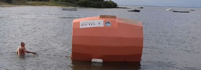
In another recent story, a Frenchman will be hoping he gets currents that move a lot faster than the ACC. Jean-Jacques Savin is attempting to cross the North Atlantic Ocean in a barrel. He set off from the Canary Islands on the 28th of December and intends to reach the Caribbean by March.

Along the way, Mr Savin will drop markers to help oceanographers from the JCOMMOPS international marine observatory study currents in the Atlantic. (Ed: you would think that the barrel itself is a big marker).

Jean-Jacques believes that ocean currents will carry him 4500 km across the Atlantic in less than 3 months. That would be an average speed of 0.5 m/s or 1.1 knots.

This seems fast. To be carried by currents alone, Jean-Jacques will have to first catch the Canary Current down the West African coast from 32 N to 20 N. This current has typical speeds of 0.1 m/s but can be up to 0.7 m/s through the Canary Islands. He would then turn west and catch the North Equatorial Current from 20 W to 65 W. This current has typical speeds of 0.1 m/s.

He will be travelling a similar distance to Wild Eyes in similar strength currents but let’s hope it doesn’t take 8.5 years.

One thing that differentiates the barrel from the capsized boat Wild Eyes is that it floats high in the water and will have significant windage. It will probably be the effective ‘sail’ of the huge barrel that will push him across the ocean, rather than the currents.

Do you think Jean-Jacques will make it to the Caribbean before his foie-gras runs out?